Background and Application

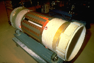
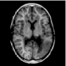
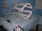
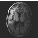
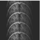
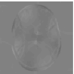
The goal of parallel imaging is to accelerate image acquisition and thereby to facilitate high temporal resolution for dynamic examinations as in DCE-MRI (dynamic contrast enhanced magnetic resonance imaging). Shown here are (1) a large body coil, (2) a body coil image measured with full sampling, (3) several surface coils, (4) a surface coil image measured with full sampling and (5) a surface coil image measured with subsampling:

(1)	(2)	(3)	(4)	(5)

Note that the fully sampled coil image in (4) is modulated in relation to the body coil image in (2). Also, the undersampled image in (5) can be acquired in less time, but suffers from aliasing. The strategy of parallel imaging is to measure less by employing a subsampling strategy but yet to use several surface coils measuring in parallel in a complementary fashion which allows to reconstruct an image such as seen in (2).

Objectives

The available data are not only modulated and aliased, but because of the higher temporal resolution required, the correspondingly reduced acquisition time per image results in a relatively high noise level. Thus, the objective is to overcome the modulations, aliasing and noise in each surface coil measurement, and to combine these data to reconstruct an underlying uncorrupted image.

Problem Formulation and Methods Used

Let {I_i} be the measured surface coil images, whose aliasing can be described by the subsampling projection P = ^-1X where denotes a Fourier Transform. The sensititity σ_i of the ith coil is estimated together with the reconstructed image I by minimizing:

where ϕ is a convex function and ν > 0. Although thus functional possesses a bilinear structure in the residual, its non-convexity makes it unsuitable for a standard Newton minimization. Convexity with respect to each isolated variable permits a duality formulation and to use Newton to solve rapidly for one variable after the other.

Results

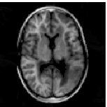
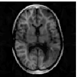
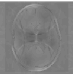
In the following example, the above method is compared with an established iteratively regularized Gauss-Newton method, where reconstructions are shown respectively in the second and third images, while the distributed errors are shown respectively in the first and fourth images. Reconstructions are performed from data simulated for 4 coils, subsampling every other horizontal and vertical line of frequencies, including only 8 additional low frequencies. Under these circumstances, the proposed reconstruction method is clearly more accurate.